SQL Query Language
Energy Logserver SQL lets you write queries in SQL rather than the Query domain-specific language (DSL). This section covers practical examples and complete SQL syntax reference.
SIEM Examples
Use SQL query to get security related data:
Example 1: Check number of failed login attempts
Query:
SELECT COUNT(sys.client.ip) AS failed_login_attempts FROM syslog-2024.02.23 sys
WHERE postfix_message = "SASL LOGIN authentication failed: UGFzc3dvcmQ6"
Result:
	failed_login_attempts
1	1329
Example 2: Gather host data from different sources in one place using JOIN
Query:
SELECT syslog.host.ip, syslog.host.name, server_addr, mac
FROM syslog-2024.02.23 syslog JOIN stream-2024.02.23 ON server_addr = syslog.host.ip
Result:
	syslog.host.ip	syslog.host.name	server_addr	mac
	192.168.10.1	   example-hostname-1	192.168.10.1	bc:24:11:0g:f9:28
	192.168.10.1	   example-hostname-1	192.168.10.1	bc:24:11:0g:f9:28
	192.168.10.2	   example-hostname-2	192.168.10.2	bs:12:18:0g:f2:66
	192.168.10.1	   example-hostname-1	192.168.10.1	bc:24:11:0g:f9:28
	192.168.10.1	   example-hostname-1	192.168.10.1	bc:24:11:0g:f9:28
Example 3: See MAC addresses and their assigned IP addresses:
Query:
POST /_plugins/_sql
{
  "query" : "SELECT mac, client_addr FROM stream-2024.02.20 WHERE netflow.type ='dhcp'"
}
Result:
{
  "schema": [
    {
      "name": "mac",
      "type": "keyword"
    },
    {
      "name": "client_addr",
      "type": "keyword"
    }
  ],
  "total": 3369,
  "datarows": [
    [
      "cs:96:d5:98:55:72",
      "10.7.7.2"
    ],
    [
      "bw:85:58:6a:b7:5a",
      "10.7.7.232"
    ],
    [
      "bc:34:11:0d:s9:88",
      "192.168.10.200"
    ]
    ]
    }
Example 4: Check total number of warnings from syslog:
Query:
SELECT COUNT(sys.syslog_severity_code) AS warnings_total FROM syslog-2024.02.23 sys
WHERE syslog_severity = "warning"
Result:
warnings_total
429822
Example 5: Check number of failed login attempts for every client:
Query:
SELECT sys.client.ip, COUNT(*) AS failed_login_attempts FROM syslog-2024.02.23 sys
WHERE  postfix_message = "SASL LOGIN authentication failed: CGZFzc3evxmQ6"
GROUP BY sys.client.ip
Result:
client.ip	failed_login_attempts
144.220.71.224	3
127.174.131.70	2
146.114.84.226	3
142.169.105.19	5
142.180.112.241	3
155.211.74.18	1
SQL in Energy Logserver bridges the gap between traditional relational database concepts and the flexibility of Energy Logserver’s document-oriented data storage. This integration gives you the ability to use your SQL knowledge to query, analyze, and extract insights from your data.
SQL and Energy Logserver terminology
Here’s how core SQL concepts map to Energy Logserver:
| SQL | {{ project }} |
|---|---|
| Table | Index |
| Row | Document |
| Column | Field |
REST API
To use the SQL plugin with your own applications, send requests to the _plugins/_sql endpoint:
POST _plugins/_sql
{
  "query": "SELECT * FROM my-index LIMIT 50"
}
You can query multiple indexes by using a comma-separated list:
POST _plugins/_sql
{
  "query": "SELECT * FROM my-index1,myindex2,myindex3 LIMIT 50"
}
You can also specify an index pattern with a wildcard expression:
POST _plugins/_sql
{
  "query": "SELECT * FROM my-index* LIMIT 50"
}
To run the above query in the command line, use the curl command:
curl -XPOST https://localhost:9200/_plugins/_sql -u 'admin:admin' -k -H 'Content-Type: application/json' -d '{"query": "SELECT * FROM my-index* LIMIT 50"}'
You can specify the response format as JDBC, standard Energy Logserver JSON, CSV, or raw. By default, queries return data in JDBC format. The following query sets the format to JSON:
POST _plugins/_sql?format=json
{
  "query": "SELECT * FROM my-index LIMIT 50"
}
See the rest of this guide for more information about request parameters, settings, supported operations, and tools.
Basic queries
Use the SELECT clause, along with FROM, WHERE, GROUP BY, HAVING, ORDER BY, and LIMIT to search and aggregate data.
Among these clauses, SELECT and FROM are required, as they specify which fields to retrieve and which indexes to retrieve them from. All other clauses are optional. Use them according to your needs.
Syntax
The complete syntax for searching and aggregating data is as follows:
SELECT [DISTINCT] (* | expression) [[AS] alias] [, ...]
FROM index_name
[WHERE predicates]
[GROUP BY expression [, ...]
 [HAVING predicates]]
[ORDER BY expression [IS [NOT] NULL] [ASC | DESC] [, ...]]
[LIMIT [offset, ] size]
Fundamentals
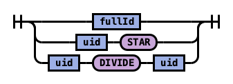
Apart from the predefined keywords of SQL, the most basic elements are literal and identifiers. A literal is a numeric, string, date or boolean constant. An identifier is an Energy Logserver index or field name. With arithmetic operators and SQL functions, use literals and identifiers to build complex expressions.
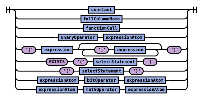
Rule expressionAtom:
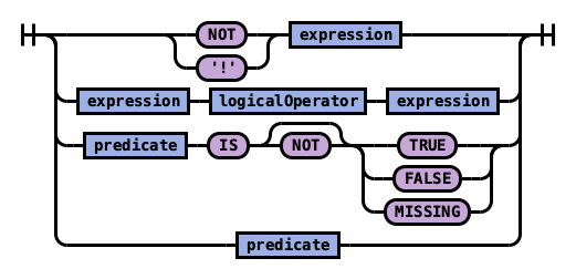
The expression in turn can be combined into a predicate with logical operator. Use a predicate in the WHERE and HAVING clause to filter out data by specific conditions.
Rule expression:
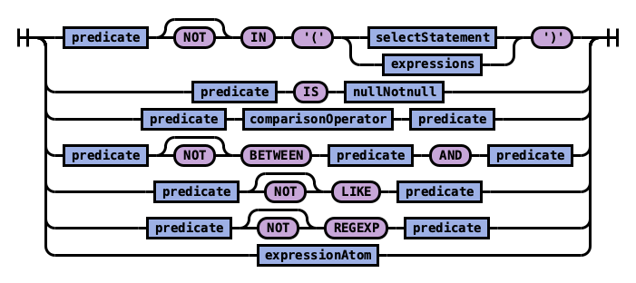
Rule predicate:
Execution Order
These SQL clauses execute in an order different from how they appear:
FROM index
 WHERE predicates
  GROUP BY expressions
   HAVING predicates
    SELECT expressions
     ORDER BY expressions
      LIMIT size
Select
Specify the fields to be retrieved.
Syntax
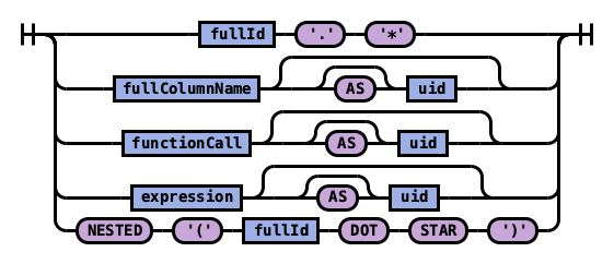
Rule selectElements:

Rule selectElement:
Example 1: Use * to retrieve all fields in an index:
SELECT *
FROM accounts
| account_number | firstname | gender | city | balance | employer | state | address | lastname | age | |
|---|---|---|---|---|---|---|---|---|---|---|
| 1 | Amber | M | Brogan | 39225 | Pyrami | IL | amberduke@pyrami.com | 880 Holmes Lane | Duke | 32 |
| 16 | Hattie | M | Dante | 5686 | Netagy | TN | hattiebond@netagy.com | 671 Bristol Street | Bond | 36 |
| 13 | Nanette | F | Nogal | 32838 | Quility | VA | nanettebates@quility.com | 789 Madison Street | Bates | 28 |
| 18 | Dale | M | Orick | 4180 | MD | daleadams@boink.com | 467 Hutchinson Court | Adams | 33 |
Example 2: Use field name(s) to retrieve only specific fields:
SELECT firstname, lastname
FROM accounts
| firstname | lastname |
|---|---|
| Amber | Duke |
| Hattie | Bond |
| Nanette | Bates |
| Dale | Adams |
Example 3: Use field aliases instead of field names. Field aliases are used to make field names more readable:
SELECT account_number AS num
FROM accounts
| num |
|---|
| 1 |
| 6 |
| 13 |
| 18 |
Example 4: Use the DISTINCT clause to get back only unique field values. You can specify one or more field names:
SELECT DISTINCT age
FROM accounts
| age |
|---|
| 28 |
| 32 |
| 33 |
| 36 |
From
Specify the index that you want search.
You can specify subqueries within the FROM clause.
Syntax
Rule tableName:
Example 1: Use index aliases to query across indexes.
In this sample query, acc is an alias for the accounts index:
SELECT account_number, accounts.age
FROM accounts
or
SELECT account_number, acc.age
FROM accounts acc
| account_number | age |
|---|---|
| 1 | 32 |
| 6 | 36 |
| 13 | 28 |
| 18 | 33 |
Example 2: Use index patterns to query indexes that match a specific pattern:
SELECT account_number
FROM account*
| account_number |
|---|
| 1 |
| 6 |
| 13 |
| 18 |
Where
Specify a condition to filter the results.
| Operators | Behavior |
|---|---|
| = | Equal to. |
| <> | Not equal to. |
| > | Greater than. |
| < | Less than. |
| >= | Greater than or equal to. |
| <= | Less than or equal to. |
| IN | Specify multiple `OR` operators. |
| BETWEEN | Similar to a range query. |
| LIKE | Use for full-text search. For more information about full-text queries. |
| IS NULL | Check if the field value is `NULL`. |
| IS NOT NULL | Check if the field value is `NOT NULL`. |
Combine comparison operators (=, <>, >, >=, <, <=) with boolean operators NOT, AND, or OR to build more complex expressions.
Example 1: Use comparison operators for numbers, strings, or dates:
SELECT account_number
FROM accounts
WHERE account_number = 1
| account_number |
|---|
| 1 |
Example 2: Energy Logserver allows for flexible schema,so documents in an index may have different fields. Use IS NULL or IS NOT NULL to retrieve only missing fields or existing fields. Energy Logserver does not differentiate between missing fields and fields explicitly set to NULL:
SELECT account_number, employer
FROM accounts
WHERE employer IS NULL
| account_number | employer |
|---|---|
| 18 |
Example 3: Deletes a document that satisfies the predicates in the WHERE clause:
DELETE FROM accounts
WHERE age > 30
Group By
Group documents with the same field value into buckets.
Example 1: Group by fields:
SELECT age
FROM accounts
GROUP BY age
| id | age |
|---|---|
| 0 | 28 |
| 1 | 32 |
| 2 | 33 |
| 3 | 36 |
Example 2: Group by field alias:
SELECT account_number AS num
FROM accounts
GROUP BY num
| id | num |
|---|---|
| 0 | 1 |
| 1 | 6 |
| 2 | 13 |
| 3 | 18 |
Example 4: Use scalar functions in the GROUP BY clause:
SELECT ABS(age) AS a
FROM accounts
GROUP BY ABS(age)
| id | a |
|---|---|
| 0 | 28.0 |
| 1 | 32.0 |
| 2 | 33.0 |
| 3 | 36.0 |
Having
Use the HAVING clause to aggregate inside each bucket based on aggregation functions (COUNT, AVG, SUM, MIN, and MAX).
The HAVING clause filters results from the GROUP BY clause:
Example 1:
SELECT age, MAX(balance)
FROM accounts
GROUP BY age HAVING MIN(balance) > 10000
| id | age | MAX (balance) |
|---|---|---|
| 0 | 28 | 32838 |
| 1 | 32 | 39225 |
Order By
Use the ORDER BY clause to sort results into your desired order.
Example 1: Use ORDER BY to sort by ascending or descending order. Besides regular field names, using ordinal, alias, or scalar functions are supported:
SELECT account_number
FROM accounts
ORDER BY account_number DESC
| account_number |
|---|
| 18 |
| 13 |
| 6 |
| 1 |
Example 2: Specify if documents with missing fields are to be put at the beginning or at the end of the results. The default behavior of Energy Logserver is to return nulls or missing fields at the end. To push them before non-nulls, use the IS NOT NULL operator:
SELECT employer
FROM accounts
ORDER BY employer IS NOT NULL
| employer |
|---|
| Netagy |
| Pyrami |
| Quility |
Limit
Specify the maximum number of documents that you want to retrieve. Used to prevent fetching large amounts of data into memory.
Example 1: If you pass in a single argument, it’s mapped to the size parameter in Energy Logserver and the from parameter is set to 0.
SELECT account_number
FROM accounts
ORDER BY account_number LIMIT 1
| account_number |
|---|
| 1 |
Example 2: If you pass in two arguments, the first is mapped to the from parameter and the second to the size parameter in Energy Logserver. You can use this for simple pagination for small indexes, as it’s inefficient for large indexes.
Use ORDER BY to ensure the same order between pages:
SELECT account_number
FROM accounts
ORDER BY account_number LIMIT 1, 1
| account_number |
|---|
| 6 |
Complex queries
Besides simple SFW (SELECT-FROM-WHERE) queries, the SQL plugin supports complex queries such as subquery, join, union, and minus. These queries operate on more than one Energy Logserver index. To examine how these queries execute behind the scenes, use the explain operation.
Joins
Energy Logserver SQL supports inner joins, cross joins, and left outer joins.
Constraints
Joins have a number of constraints:
You can only join two indexes.
You must use aliases for indexes (for example,
people p).Within an ON clause, you can only use AND conditions.
In a WHERE statement, don’t combine trees that contain multiple indexes. For example, the following statement works:
WHERE (a.type1 > 3 OR a.type1 < 0) AND (b.type2 > 4 OR b.type2 < -1)
The following statement does not:
WHERE (a.type1 > 3 OR b.type2 < 0) AND (a.type1 > 4 OR b.type2 < -1)
You can’t use GROUP BY or ORDER BY for results.
LIMIT with OFFSET (e.g.
LIMIT 25 OFFSET 25) is not supported.
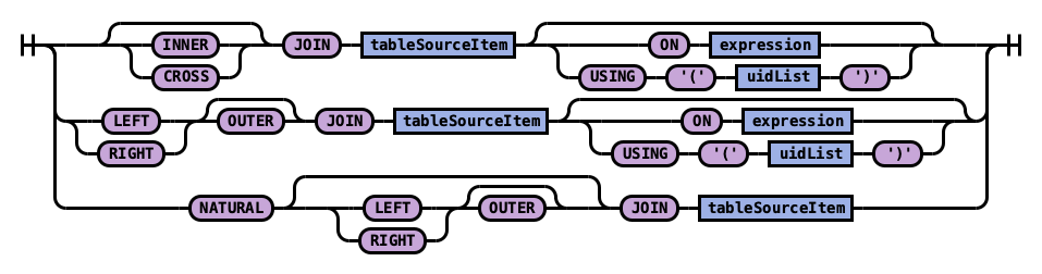
Description
The JOIN clause combines columns from one or more indexes using values common to each.
Syntax
Rule tableSource:

Rule joinPart:
Example 1: Inner join
Inner join creates a new result set by combining columns of two indexes based on your join predicates. It iterates the two indexes and compares each document to find the ones that satisfy the join predicates. You can optionally precede the JOIN clause with an INNER keyword.
The join predicate(s) is specified by the ON clause.
SQL query:
SELECT
  a.account_number, a.firstname, a.lastname,
  e.id, e.name
FROM accounts a
JOIN employees_nested e
 ON a.account_number = e.id
Explain:
The explain output is complicated, because a JOIN clause is associated with two Energy Logserver DSL queries that execute in separate query planner frameworks. You can interpret it by examining the Physical Plan and Logical Plan objects.
{
  "Physical Plan" : {
    "Project [ columns=[a.account_number, a.firstname, a.lastname, e.name, e.id] ]" : {
      "Top [ count=200 ]" : {
        "BlockHashJoin[ conditions=( a.account_number = e.id ), type=JOIN, blockSize=[FixedBlockSize with size=10000] ]" : {
          "Scroll [ employees_nested as e, pageSize=10000 ]" : {
            "request" : {
              "size" : 200,
              "from" : 0,
              "_source" : {
                "excludes" : [ ],
                "includes" : [
                  "id",
                  "name"
                ]
              }
            }
          },
          "Scroll [ accounts as a, pageSize=10000 ]" : {
            "request" : {
              "size" : 200,
              "from" : 0,
              "_source" : {
                "excludes" : [ ],
                "includes" : [
                  "account_number",
                  "firstname",
                  "lastname"
                ]
              }
            }
          },
          "useTermsFilterOptimization" : false
        }
      }
    }
  },
  "description" : "Hash Join algorithm builds hash table based on result of first query, and then probes hash table to find matched rows for each row returned by second query",
  "Logical Plan" : {
    "Project [ columns=[a.account_number, a.firstname, a.lastname, e.name, e.id] ]" : {
      "Top [ count=200 ]" : {
        "Join [ conditions=( a.account_number = e.id ) type=JOIN ]" : {
          "Group" : [
            {
              "Project [ columns=[a.account_number, a.firstname, a.lastname] ]" : {
                "TableScan" : {
                  "tableAlias" : "a",
                  "tableName" : "accounts"
                }
              }
            },
            {
              "Project [ columns=[e.name, e.id] ]" : {
                "TableScan" : {
                  "tableAlias" : "e",
                  "tableName" : "employees_nested"
                }
              }
            }
          ]
        }
      }
    }
  }
}
Result set:
| a.account_number | a.firstname | a.lastname | e.id | e.name |
|---|---|---|---|---|
| 6 | Hattie | Bond | 6 | Jane Smith |
Example 2: Cross join
Cross join, also known as cartesian join, combines each document from the first index with each document from the second.
The result set is the cartesian product of documents of both indexes.
This operation is similar to the inner join without the ON clause that specifies the join condition.
Warning
It’s risky to perform cross join on two indexes of large or even medium size. It might trigger a circuit breaker that terminates the query to avoid running out of memory.
SQL query:
SELECT
  a.account_number, a.firstname, a.lastname,
  e.id, e.name
FROM accounts a
JOIN employees_nested e
Result set:
| a.account_number | a.firstname | a.lastname | e.id | e.name |
|---|---|---|---|---|
| 1 | Amber | Duke | 3 | Bob Smith |
| 1 | Amber | Duke | 4 | Susan Smith |
| 1 | Amber | Duke | 6 | Jane Smith |
| 6 | Hattie | Bond | 3 | Bob Smith |
| 6 | Hattie | Bond | 4 | Susan Smith |
| 6 | Hattie | Bond | 6 | Jane Smith |
| 13 | Nanette | Bates | 3 | Bob Smith |
| 13 | Nanette | Bates | 4 | Susan Smith |
| 13 | Nanette | Bates | 6 | Jane Smith |
| 18 | Dale | Adams | 3 | Bob Smith |
| 18 | Dale | Adams | 4 | Susan Smith |
| 18 | Dale | Adams | 6 | Jane Smith |
Example 3: Left outer join
Use left outer join to retain rows from the first index if it does not satisfy the join predicate. The keyword OUTER is optional.
SQL query:
SELECT
  a.account_number, a.firstname, a.lastname,
  e.id, e.name
FROM accounts a
LEFT JOIN employees_nested e
 ON a.account_number = e.id
Result set:
| a.account_number | a.firstname | a.lastname | e.id | e.name |
|---|---|---|---|---|
| 1 | Amber | Duke | null | null |
| 6 | Hattie | Bond | 6 | Jane Smith |
| 13 | Nanette | Bates | null | null |
| 18 | Dale | Adams | null | null |
Subquery
A subquery is a complete SELECT statement used within another statement and enclosed in parenthesis.
From the explain output, you can see that some subqueries are actually transformed to an equivalent join query to execute.
Example 1: Table subquery
SQL query:
SELECT a1.firstname, a1.lastname, a1.balance
FROM accounts a1
WHERE a1.account_number IN (
  SELECT a2.account_number
  FROM accounts a2
  WHERE a2.balance > 10000
)
Explain:
{
  "Physical Plan" : {
    "Project [ columns=[a1.balance, a1.firstname, a1.lastname] ]" : {
      "Top [ count=200 ]" : {
        "BlockHashJoin[ conditions=( a1.account_number = a2.account_number ), type=JOIN, blockSize=[FixedBlockSize with size=10000] ]" : {
          "Scroll [ accounts as a2, pageSize=10000 ]" : {
            "request" : {
              "size" : 200,
              "query" : {
                "bool" : {
                  "filter" : [
                    {
                      "bool" : {
                        "adjust_pure_negative" : true,
                        "must" : [
                          {
                            "bool" : {
                              "adjust_pure_negative" : true,
                              "must" : [
                                {
                                  "bool" : {
                                    "adjust_pure_negative" : true,
                                    "must_not" : [
                                      {
                                        "bool" : {
                                          "adjust_pure_negative" : true,
                                          "must_not" : [
                                            {
                                              "exists" : {
                                                "field" : "account_number",
                                                "boost" : 1
                                              }
                                            }
                                          ],
                                          "boost" : 1
                                        }
                                      }
                                    ],
                                    "boost" : 1
                                  }
                                },
                                {
                                  "range" : {
                                    "balance" : {
                                      "include_lower" : false,
                                      "include_upper" : true,
                                      "from" : 10000,
                                      "boost" : 1,
                                      "to" : null
                                    }
                                  }
                                }
                              ],
                              "boost" : 1
                            }
                          }
                        ],
                        "boost" : 1
                      }
                    }
                  ],
                  "adjust_pure_negative" : true,
                  "boost" : 1
                }
              },
              "from" : 0
            }
          },
          "Scroll [ accounts as a1, pageSize=10000 ]" : {
            "request" : {
              "size" : 200,
              "from" : 0,
              "_source" : {
                "excludes" : [ ],
                "includes" : [
                  "firstname",
                  "lastname",
                  "balance",
                  "account_number"
                ]
              }
            }
          },
          "useTermsFilterOptimization" : false
        }
      }
    }
  },
  "description" : "Hash Join algorithm builds hash table based on result of first query, and then probes hash table to find matched rows for each row returned by second query",
  "Logical Plan" : {
    "Project [ columns=[a1.balance, a1.firstname, a1.lastname] ]" : {
      "Top [ count=200 ]" : {
        "Join [ conditions=( a1.account_number = a2.account_number ) type=JOIN ]" : {
          "Group" : [
            {
              "Project [ columns=[a1.balance, a1.firstname, a1.lastname, a1.account_number] ]" : {
                "TableScan" : {
                  "tableAlias" : "a1",
                  "tableName" : "accounts"
                }
              }
            },
            {
              "Project [ columns=[a2.account_number] ]" : {
                "Filter [ conditions=[AND ( AND account_number ISN null, AND balance GT 10000 ) ] ]" : {
                  "TableScan" : {
                    "tableAlias" : "a2",
                    "tableName" : "accounts"
                  }
                }
              }
            }
          ]
        }
      }
    }
  }
}
Result set:
| a1.firstname | a1.lastname | a1.balance |
|---|---|---|
| Amber | Duke | 39225 |
| Nanette | Bates | 32838 |
Example 2: From subquery
SQL query:
SELECT a.f, a.l, a.a
FROM (
  SELECT firstname AS f, lastname AS l, age AS a
  FROM accounts
  WHERE age > 30
) AS a
Explain:
{
  "from" : 0,
  "size" : 200,
  "query" : {
    "bool" : {
      "filter" : [
        {
          "bool" : {
            "must" : [
              {
                "range" : {
                  "age" : {
                    "from" : 30,
                    "to" : null,
                    "include_lower" : false,
                    "include_upper" : true,
                    "boost" : 1.0
                  }
                }
              }
            ],
            "adjust_pure_negative" : true,
            "boost" : 1.0
          }
        }
      ],
      "adjust_pure_negative" : true,
      "boost" : 1.0
    }
  },
  "_source" : {
    "includes" : [
      "firstname",
      "lastname",
      "age"
    ],
    "excludes" : [ ]
  }
}
Result set:
| f | l | a |
|---|---|---|
| Amber | Duke | 32 |
| Dale | Adams | 33 |
| Hattie | Bond | 36 |
Functions
The SQL language supports all SQL plugin common functions, including relevance search, but also introduces a few function synonyms, which are available in SQL only.
These synonyms are provided by the V1 engine.
Match query
The MATCHQUERY and MATCH_QUERY functions are synonyms for the MATCH relevance function. They don’t accept additional arguments but provide an alternate syntax.
Syntax
To use matchquery or match_query, pass in your search query and the field name that you want to search against:
match_query(field_expression, query_expression[, option=<option_value>]*)
matchquery(field_expression, query_expression[, option=<option_value>]*)
field_expression = match_query(query_expression[, option=<option_value>]*)
field_expression = matchquery(query_expression[, option=<option_value>]*)
You can specify the following options in any order:
analyzerboost
Example
You can use MATCHQUERY to replace MATCH:
SELECT account_number, address
FROM accounts
WHERE MATCHQUERY(address, 'Holmes')
Alternatively, you can use MATCH_QUERY to replace MATCH:
SELECT account_number, address
FROM accounts
WHERE address = MATCH_QUERY('Holmes')
The results contain documents in which the address contains “Holmes”:
| account_number | address |
|---|---|
| 1 | 880 Holmes Lane |
Multi-match
There are three synonyms for MULTI_MATCH, each with a slightly different syntax. They accept a query string and a fields list with weights. They can also accept additional optional parameters.
Syntax
multimatch('query'=query_expression[, 'fields'=field_expression][, option=<option_value>]*)
multi_match('query'=query_expression[, 'fields'=field_expression][, option=<option_value>]*)
multimatchquery('query'=query_expression[, 'fields'=field_expression][, option=<option_value>]*)
The fields parameter is optional and can contain a single field or a comma-separated list (whitespace characters are not allowed). The weight for each field is optional and is specified after the field name. It should be delimited by the caret character – ^ – without whitespace.
Example
The following queries show the fields parameter of a multi-match query with a single field and a field list:
multi_match('fields' = "Tags^2,Title^3.4,Body,Comments^0.3", ...)
multi_match('fields' = "Title", ...)
You can specify the following options in any order:
analyzerboostsloptypetie_breakeroperator
Query string
The QUERY function is a synonym for QUERY_STRING.
Syntax
query('query'=query_expression[, 'fields'=field_expression][, option=<option_value>]*)
The fields parameter is optional and can contain a single field or a comma-separated list (whitespace characters are not allowed). The weight for each field is optional and is specified after the field name. It should be delimited by the caret character – ^ – without whitespace.
Example
The following queries show the fields parameter of a multi-match query with a single field and a field list:
query('fields' = "Tags^2,Title^3.4,Body,Comments^0.3", ...)
query('fields' = "Tags", ...)
You can specify the following options in any order:
analyzerboostslopdefault_field
Example of using query_string in SQL and PPL queries:
The following is a sample REST API search request in Energy Logserver DSL.
GET accounts/_search
{
  "query": {
    "query_string": {
      "query": "Lane Street",
      "fields": [ "address" ],
    }
  }
}
The request above is equivalent to the following query function:
SELECT account_number, address
FROM accounts
WHERE query('address:Lane OR address:Street')
The results contain addresses that contain “Lane” or “Street”:
| account_number | address |
|---|---|
| 1 | 880 Holmes Lane |
| 6 | 671 Bristol Street |
| 13 | 789 Madison Street |
Match phrase
The MATCHPHRASEQUERY function is a synonym for MATCH_PHRASE.
Syntax
matchphrasequery(query_expression, field_expression[, option=<option_value>]*)
You can specify the following options in any order:
analyzerboostslop
Score query
To return a relevance score along with every matching document, use the SCORE, SCOREQUERY, or SCORE_QUERY functions.
Syntax
The SCORE function expects two arguments. The first argument is the MATCH_QUERY expression. The second argument is an optional floating-point number to boost the score (the default value is 1.0):
SCORE(match_query_expression, score)
SCOREQUERY(match_query_expression, score)
SCORE_QUERY(match_query_expression, score)
Example
The following example uses the SCORE function to boost the documents’ scores:
SELECT account_number, address, _score
FROM accounts
WHERE SCORE(MATCH_QUERY(address, 'Lane'), 0.5) OR
  SCORE(MATCH_QUERY(address, 'Street'), 100)
ORDER BY _score
The results contain matches with corresponding scores:
| account_number | address | score |
|---|---|---|
| 1 | 880 Holmes Lane | 0.5 |
| 6 | 671 Bristol Street | 100 |
| 13 | 789 Madison Street | 100 |
Wildcard query
To search documents by a given wildcard, use the WILDCARDQUERY or WILDCARD_QUERY functions.
Syntax
wildcardquery(field_expression, query_expression[, boost=<value>])
wildcard_query(field_expression, query_expression[, boost=<value>])
Example
The following example uses a wildcard query:
SELECT account_number, address
FROM accounts
WHERE wildcard_query(address, '*Holmes*');
The results contain documents that match the wildcard expression:
account_number |
address |
|---|---|
1 |
880 Holmes Lane |
JSON Support
SQL plugin supports JSON by following PartiQL specification, a SQL-compatible query language that lets you query semi-structured and nested data for any data format. The SQL plugin only supports a subset of the PartiQL specification.
Querying nested collection
PartiQL extends SQL to allow you to query and unnest nested collections. In Energy Logserver, this is very useful to query a JSON index with nested objects or fields.
To follow along, use the bulk operation to index some sample data:
POST employees_nested/_bulk?refresh
{"index":{"_id":"1"}}
{"id":3,"name":"Bob Smith","title":null,"projects":[{"name":"SQL Spectrum querying","started_year":1990},{"name":"SQL security","started_year":1999},{"name":"{{ project }} security","started_year":2015}]}
{"index":{"_id":"2"}}
{"id":4,"name":"Susan Smith","title":"Dev Mgr","projects":[]}
{"index":{"_id":"3"}}
{"id":6,"name":"Jane Smith","title":"Software Eng 2","projects":[{"name":"SQL security","started_year":1998},{"name":"Hello security","started_year":2015,"address":[{"city":"Dallas","state":"TX"}]}]}
Example 1: Unnesting a nested collection
This example finds the nested document (projects) with a field value (name) that satisfies the predicate (contains security). Because each parent document can have more than one nested documents, the nested document that matches is flattened. In other words, the final result is the cartesian product between the parent and nested documents.
SELECT e.name AS employeeName,
       p.name AS projectName
FROM employees_nested AS e,
       e.projects AS p
WHERE p.name LIKE '%security%'
Explain:
{
  "from" : 0,
  "size" : 200,
  "query" : {
    "bool" : {
      "filter" : [
        {
          "bool" : {
            "must" : [
              {
                "nested" : {
                  "query" : {
                    "wildcard" : {
                      "projects.name" : {
                        "wildcard" : "*security*",
                        "boost" : 1.0
                      }
                    }
                  },
                  "path" : "projects",
                  "ignore_unmapped" : false,
                  "score_mode" : "none",
                  "boost" : 1.0,
                  "inner_hits" : {
                    "ignore_unmapped" : false,
                    "from" : 0,
                    "size" : 3,
                    "version" : false,
                    "seq_no_primary_term" : false,
                    "explain" : false,
                    "track_scores" : false,
                    "_source" : {
                      "includes" : [
                        "projects.name"
                      ],
                      "excludes" : [ ]
                    }
                  }
                }
              }
            ],
            "adjust_pure_negative" : true,
            "boost" : 1.0
          }
        }
      ],
      "adjust_pure_negative" : true,
      "boost" : 1.0
    }
  },
  "_source" : {
    "includes" : [
      "name"
    ],
    "excludes" : [ ]
  }
}
Result set:
| employeeName | projectName |
|---|---|
| Bob Smith | {{ project }} Security |
| Bob Smith | SQL security |
| Jane Smith | Hello security |
| Jane Smith | SQL security |
Example 2: Unnesting in existential subquery
To unnest a nested collection in a subquery to check if it satisfies a condition:
SELECT e.name AS employeeName
FROM employees_nested AS e
WHERE EXISTS (
    SELECT *
    FROM e.projects AS p
    WHERE p.name LIKE '%security%'
)
Explain:
{
  "from" : 0,
  "size" : 200,
  "query" : {
    "bool" : {
      "filter" : [
        {
          "bool" : {
            "must" : [
              {
                "nested" : {
                  "query" : {
                    "bool" : {
                      "must" : [
                        {
                          "bool" : {
                            "must" : [
                              {
                                "bool" : {
                                  "must_not" : [
                                    {
                                      "bool" : {
                                        "must_not" : [
                                          {
                                            "exists" : {
                                              "field" : "projects",
                                              "boost" : 1.0
                                            }
                                          }
                                        ],
                                        "adjust_pure_negative" : true,
                                        "boost" : 1.0
                                      }
                                    }
                                  ],
                                  "adjust_pure_negative" : true,
                                  "boost" : 1.0
                                }
                              },
                              {
                                "wildcard" : {
                                  "projects.name" : {
                                    "wildcard" : "*security*",
                                    "boost" : 1.0
                                  }
                                }
                              }
                            ],
                            "adjust_pure_negative" : true,
                            "boost" : 1.0
                          }
                        }
                      ],
                      "adjust_pure_negative" : true,
                      "boost" : 1.0
                    }
                  },
                  "path" : "projects",
                  "ignore_unmapped" : false,
                  "score_mode" : "none",
                  "boost" : 1.0
                }
              }
            ],
            "adjust_pure_negative" : true,
            "boost" : 1.0
          }
        }
      ],
      "adjust_pure_negative" : true,
      "boost" : 1.0
    }
  },
  "_source" : {
    "includes" : [
      "name"
    ],
    "excludes" : [ ]
  }
}
Result set:
| employeeName | :— | :— Bob Smith | Jane Smith |
Metadata queries
To see basic metadata about your indexes, use the SHOW and DESCRIBE commands.
Syntax
Rule showStatement:

Rule showFilter:

Example 1: See metadata for indexes
To see metadata for indexes that match a specific pattern, use the SHOW command.
Use the wildcard % to match all indexes:
SHOW TABLES LIKE %
| TABLE_CAT | TABLE_SCHEM | TABLE_NAME | TABLE_TYPE | REMARKS | TYPE_CAT | TYPE_SCHEM | TYPE_NAME | SELF_REFERENCING_COL_NAME | REF_GENERATION :— | :— docker-cluster | null | accounts | BASE TABLE | null | null | null | null | null | null docker-cluster | null | employees_nested | BASE TABLE | null | null | null | null | null | null
Example 2: See metadata for a specific index
To see metadata for an index name with a prefix of acc:
SHOW TABLES LIKE acc%
| TABLE_CAT | TABLE_SCHEM | TABLE_NAME | TABLE_TYPE | REMARKS | TYPE_CAT | TYPE_SCHEM | TYPE_NAME | SELF_REFERENCING_COL_NAME | REF_GENERATION :— | :— docker-cluster | null | accounts | BASE TABLE | null | null | null | null | null | null
Example 3: See metadata for fields
To see metadata for field names that match a specific pattern, use the DESCRIBE command:
DESCRIBE TABLES LIKE accounts
| TABLE_CAT | TABLE_SCHEM | TABLE_NAME | COLUMN_NAME | DATA_TYPE | TYPE_NAME | COLUMN_SIZE | BUFFER_LENGTH | DECIMAL_DIGITS | NUM_PREC_RADIX | NULLABLE | REMARKS | COLUMN_DEF | SQL_DATA_TYPE | SQL_DATETIME_SUB | CHAR_OCTET_LENGTH | ORDINAL_POSITION | IS_NULLABLE | SCOPE_CATALOG | SCOPE_SCHEMA | SCOPE_TABLE | SOURCE_DATA_TYPE | IS_AUTOINCREMENT | IS_GENERATEDCOLUMN :— | :— | :— | :— | :— | :— | :— | :— | :— | :— | :— | :— | :— | :— | :— | :— | :— | :— | :— | :— | :— | :— | :— docker-cluster | null | accounts | account_number | null | long | null | null | null | 10 | 2 | null | null | null | null | null | 1 | | null | null | null | null | NO | docker-cluster | null | accounts | firstname | null | text | null | null | null | 10 | 2 | null | null | null | null | null | 2 | | null | null | null | null | NO | docker-cluster | null | accounts | address | null | text | null | null | null | 10 | 2 | null | null | null | null | null | 3 | | null | null | null | null | NO | docker-cluster | null | accounts | balance | null | long | null | null | null | 10 | 2 | null | null | null | null | null | 4 | | null | null | null | null | NO | docker-cluster | null | accounts | gender | null | text | null | null | null | 10 | 2 | null | null | null | null | null | 5 | | null | null | null | null | NO | docker-cluster | null | accounts | city | null | text | null | null | null | 10 | 2 | null | null | null | null | null | 6 | | null | null | null | null | NO | docker-cluster | null | accounts | employer | null | text | null | null | null | 10 | 2 | null | null | null | null | null | 7 | | null | null | null | null | NO | docker-cluster | null | accounts | state | null | text | null | null | null | 10 | 2 | null | null | null | null | null | 8 | | null | null | null | null | NO | docker-cluster | null | accounts | age | null | long | null | null | null | 10 | 2 | null | null | null | null | null | 9 | | null | null | null | null | NO | docker-cluster | null | accounts | email | null | text | null | null | null | 10 | 2 | null | null | null | null | null | 10 | | null | null | null | null | NO | docker-cluster | null | accounts | lastname | null | text | null | null | null | 10 | 2 | null | null | null | null | null | 11 | | null | null | null | null | NO |
Aggregate functions
Aggregate functions operate on subsets defined by the GROUP BY clause. In the absence of a GROUP BY clause, aggregate functions operate on all elements of the result set. You can use aggregate functions in the GROUP BY, SELECT, and HAVING clauses.
Energy Logserver supports the following aggregate functions.
Function |
Description |
|---|---|
|
Returns the average of the results. |
|
Returns the number of results. |
|
Returns the sum of the results. |
|
Returns the minimum of the results. |
|
Returns the maximum of the results. |
|
Returns the population variance of the results after discarding nulls. Returns 0 when there is only one row of results. |
|
Returns the sample variance of the results after discarding nulls. Returns null when there is only one row of results. |
|
Returns the sample standard deviation of the results. Returns 0 when there is only one row of results. |
|
Returns the population standard deviation of the results. Returns 0 when there is only one row of results. |
|
Returns the sample standard deviation of the results. Returns null when there is only one row of results. |
The examples below reference an employees table. You can try out the examples by indexing the following documents into Energy Logserver using the bulk index operation:
PUT employees/_bulk?refresh
{"index":{"_id":"1"}}
{"employee_id": 1, "department":1, "firstname":"Amber", "lastname":"Duke", "sales":1356, "sale_date":"2020-01-23"}
{"index":{"_id":"2"}}
{"employee_id": 1, "department":1, "firstname":"Amber", "lastname":"Duke", "sales":39224, "sale_date":"2021-01-06"}
{"index":{"_id":"6"}}
{"employee_id":6, "department":1, "firstname":"Hattie", "lastname":"Bond", "sales":5686, "sale_date":"2021-06-07"}
{"index":{"_id":"7"}}
{"employee_id":6, "department":1, "firstname":"Hattie", "lastname":"Bond", "sales":12432, "sale_date":"2022-05-18"}
{"index":{"_id":"13"}}
{"employee_id":13,"department":2, "firstname":"Nanette", "lastname":"Bates", "sales":32838, "sale_date":"2022-04-11"}
{"index":{"_id":"18"}}
{"employee_id":18,"department":2, "firstname":"Dale", "lastname":"Adams", "sales":4180, "sale_date":"2022-11-05"}
GROUP BY (Aggregate functions)
The GROUP BY clause defines subsets of a result set. Aggregate functions operate on these subsets and return one result row for each subset.
You can use an identifier, ordinal, or expression in the GROUP BY clause.
Using an identifier in GROUP BY
You can specify the field name (column name) to aggregate on in the GROUP BY clause. For example, the following query returns the department numbers and the total sales for each department:
SELECT department, sum(sales)
FROM employees
GROUP BY department;
| department | sum(sales) |
|---|---|
| 1 | 58700< |
| 2 | 37018 |
Using an ordinal in GROUP BY
You can specify the column number to aggregate on in the GROUP BY clause. The column number is determined by the column position in the SELECT clause. For example, the following query is equivalent to the query above. It returns the department numbers and the total sales for each department. It groups the results by the first column of the result set, which is department:
SELECT department, sum(sales)
FROM employees
GROUP BY 1;
| department | sum(sales) |
|---|---|
| 1 | 58700 |
| 2 | 37018 |
Using an expression in GROUP BY
You can use an expression in the GROUP BY clause. For example, the following query returns the average sales for each year:
SELECT year(sale_date), avg(sales)
FROM employees
GROUP BY year(sale_date);
| year(start_date) | avg(sales) |
|---|---|
| 2020 | 1356.0 |
| 2021 | 22455.0 |
| 2022 | 16484.0 |
SELECT (Aggregate functions)
You can use aggregate expressions in the SELECT clause either directly or as part of a larger expression. In addition, you can use expressions as arguments of aggregate functions.
Using aggregate expressions directly in SELECT
The following query returns the average sales for each department:
SELECT department, avg(sales)
FROM employees
GROUP BY department;
| department | avg(sales) |
|---|---|
| 1 | 14675.0 |
| 2 | 18509.0 |
Using aggregate expressions as part of larger expressions in SELECT
The following query calculates the average commission for the employees of each department as 5% of the average sales:
SELECT department, avg(sales) * 0.05 as avg_commission
FROM employees
GROUP BY department;
| department | avg_commission |
|---|---|
| 1 | 733.75 |
| 2 | 925.45 |
Using expressions as arguments to aggregate functions
The following query calculates the average commission amount for each department. First it calculates the commission amount for each sales value as 5% of the sales. Then it determines the average of all commission values:
SELECT department, avg(sales * 0.05) as avg_commission
FROM employees
GROUP BY department;
| department | avg_commission |
|---|---|
| 1 | 733.75 |
| 2 | 925.45 |
COUNT
The COUNT function accepts arguments, such as *, or literals, such as 1.
The following table describes how various forms of the COUNT function operate.
| Function type | Description |
|---|---|
| COUNT(field) | Counts the number of rows where the value of the given field (or expression) is not null. |
| COUNT(*) | Counts the total number of rows in a table. |
| COUNT(1) [same as COUNT(*)] | Counts any non-null literal. |
For example, the following query returns the count of sales for each year:
SELECT year(sale_date), count(sales)
FROM employees
GROUP BY year(sale_date);
| year(sale_date) | count(sales) |
|---|---|
| 2020 | 1 |
| 2021 | 2 |
| 2022 | 3 |
HAVING (Aggregate functions)
Both WHERE and HAVING are used to filter results. The WHERE filter is applied before the GROUP BY phase, so you cannot use aggregate functions in a WHERE clause. However, you can use the WHERE clause to limit the rows to which the aggregate is then applied.
The HAVING filter is applied after the GROUP BY phase, so you can use the HAVING clause to limit the groups that are included in the results.
HAVING with GROUP BY
You can use aggregate expressions or their aliases defined in a SELECT clause in a HAVING condition.
The following query uses an aggregate expression in the HAVING clause. It returns the number of sales for each employee who made more than one sale:
SELECT employee_id, count(sales)
FROM employees
GROUP BY employee_id
HAVING count(sales) > 1;
| employee_id | count(sales) |
|---|---|
| 1 | 2 |
| 6 | 2 |
The aggregations in a HAVING clause do not have to be the same as the aggregations in a SELECT list. The following query uses the count function in the HAVING clause but the sum function in the SELECT clause. It returns the total sales amount for each employee who made more than one sale:
SELECT employee_id, sum(sales)
FROM employees
GROUP BY employee_id
HAVING count(sales) > 1;
| employee_id | sum (sales) |
|---|---|
| 1 | 40580 |
| 6 | 18120 |
As an extension of the SQL standard, you are not restricted to using only identifiers in the GROUP BY clause. The following query uses an alias in the GROUP BY clause and is equivalent to the previous query:
SELECT employee_id as id, sum(sales)
FROM employees
GROUP BY id
HAVING count(sales) > 1;
| id | sum (sales) |
|---|---|
| 1 | 40580 |
| 6 | 18120 |
You can also use an alias for an aggregate expression in the HAVING clause. The following query returns the total sales for each department where sales exceed $40,000:
SELECT department, sum(sales) as total
FROM employees
GROUP BY department
HAVING total > 40000;
| department | total |
|---|---|
| 1 | 58700 |
If an identifier is ambiguous (for example, present both as a SELECT alias and as an index field), the preference is given to the alias. In the following query the identifier is replaced with the expression aliased in the SELECT clause:
SELECT department, sum(sales) as sales
FROM employees
GROUP BY department
HAVING sales > 40000;
| department | sales |
|---|---|
| 1 | 58700 |
HAVING without GROUP BY
You can use a HAVING clause without a GROUP BY clause. In this case, the whole set of data is to be considered one group. The following query will return True if there is more than one value in the department column:
SELECT 'True' as more_than_one_department FROM employees HAVING min(department) < max(department);
| more_than_one_department |
|---|
| True |
If all employees in the employee table belonged to the same department, the result would contain zero rows:
| more_than_one_department |
|---|
Delete
The DELETE statement deletes documents that satisfy the predicates in the WHERE clause.
If you don’t specify the WHERE clause, all documents are deleted.
Setting
The DELETE statement is disabled by default. To enable the DELETE functionality in SQL, you need to update the configuration by sending the following request:
PUT _plugins/_query/settings
{
  "transient": {
    "plugins.sql.delete.enabled": "true"
  }
}
Syntax
Rule singleDeleteStatement:

Example
SQL query:
DELETE FROM accounts
WHERE age > 30
Explain:
{
  "size" : 1000,
  "query" : {
    "bool" : {
      "must" : [
        {
          "range" : {
            "age" : {
              "from" : 30,
              "to" : null,
              "include_lower" : false,
              "include_upper" : true,
              "boost" : 1.0
            }
          }
        }
      ],
      "adjust_pure_negative" : true,
      "boost" : 1.0
    }
  },
  "_source" : false
}
Result set:
{
  "schema" : [
    {
      "name" : "deleted_rows",
      "type" : "long"
    }
  ],
  "total" : 1,
  "datarows" : [
    [
      3
    ]
  ],
  "size" : 1,
  "status" : 200
}
The datarows field shows the number of documents deleted.